Analysis
Data analysis and preprocessing for MRI/fMRI typically is performed using a VDI, often accessing files stored in Lagringshotell or within TSD using its own VDI, while accessing files also stored there. The lab engineer can be contacted for more information about how to connect and use VDI.
VDI – Virtual Desktop Infrastructure. A VDI offers users access to a virtual computer with the software and processing power they need. This computer can be used in the same way you use your local computer but can be reached from different devices and operating systems. Which programs that are mounted and can run on the VDI machine is decided together by yourself, your local IT and program managers at the departments. A VDI may offer advantages over using one’s office desktop computer for analysis, as the VDI processing capabilities are more powerful.
Software
Several programs have been developed by the neuroimaging community to analyze MRI/fMRI data. These different programs and toolboxes often have different goals, strengths and weaknesses that must be considered prior to deciding which one to use. Some of these decisions will be based upon a researcher’s personal preference, others will be strategic and based upon the study’s specific needs. The open-access nature of some of the programs may also lead researchers to choose one type of software over another. Some researchers additionally opt to run some parts of their preprocessing and analysis using in-house written code.
The following sections will first outline the different steps involved in preprocessing, and then continue with an overview of some of the most commonly used programs employed in preprocessing and analysis, their data outputs and structures.
Preprocessing
fMRI data is inherently noisy. As a result, a number of preprocessing steps must be performed to prepare your data prior to analysis. Preprocessing creates a 4D dataset (the 4th dimension being time) from what begins as a 3D dataset. It also improves the signal to noise ratio. Some steps are also performed to anonymize the data, improve localization within subjects by co-registering the T1 to the structural images and across subjects by warping the images to fit a universal template. These steps can be carried out in many of the same programs which are used to analyze the data. Each step will create its own output file, which varies slightly depending on the program, but the output is usually a new NIfTI file.
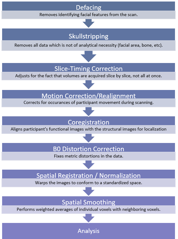
It is important to remember that different researchers, as well as different software, may perform these preprocessing tasks in an order that differs from the visual on the previous page. In some cases, researchers may choose not to employ some preprocessing steps. These decisions are ultimately made based on the study’s needs. The following section will provide a brief description of the various steps involved in preprocessing of fMRI data and their purpose.
Defacing and Skull-stripping
One method of ensuring anonymization of fMRI data is by using defacing software. Defacing software removes the voxels associated with facial features or makes them unreadable. One concern is that some of the algorithms used in defacing may inadvertently remove data relevant to a study’s purpose (Bischoff-Grethe et al., 2007). Some investigators will prefer not to deface the data because of this.
Similarly, skull-stripping, or brain extraction, removes all voxels that are not necessary for analysis, leaving just the brain, without bone, dura, surrounding air, etc. While this is yet another way of ensuring that the data is anonymized, as well as cutting down on the amount of space the data takes up in storage, not all researchers will choose to perform this step for many of the same reasons as defacing. It is essential to conduct a quality check to ensure the extraction results are precise if they are used.
Artifact-correcting Preprocessing Steps
There are several sources that can contribute to noise and artefacts in fMRI data. Steps can be taken when developing protocols such as making adjustments to TE (time to echo), TR (time to repeat), carefully planning which sequences are used, and adjusting parameters (such as slice thickness or field of view) in order to reduce noise and artefacts (Bell & Yeung et al., 2019). Some noise and artefacts, however, will inevitably need to be dealt with after the images are acquired. This can be accomplished during the preprocessing phase.
Motion correction/realignment. This step corrects for any movement that participants may have made in the scanner by aligning all of the functional images with one reference image (often the first or mid-point image). It is important to check the data carefully after this step.
Slice-timing correction. fMRI analysis assumes that all slices in a volume were taken simultaneously. This, however, is not the case. This step corrects for the fact that each slice from the total volume is taken at a different point time due to the nature of MRI data collection and adjusts for the slight delay.
B0 distortion correction. This step corrects distortions that result due to the B0 magnetic field inhomogeneity.

Spatial Preprocessing Steps
There are several sources that can contribute to noise and artefacts in fMRI data. The following steps are used to correct these issues.
Coregistration. In this step, the T1 and/or T2 structural images are used for coregistration of the functional scans so that the functional images align with the anatomical structures/brain regions of the participant.
Spatial Normalization. Human brains can have significant variations from one participant to the next. Thus, when comparing subjects, it is important to ensure that all of the data conforms to the same space so that a voxel in one subject represents the same location compared to another subject. This is achieved by warping the data to a template/atlas brain. This step is necessary to second level analysis in order to compare across participants.
Spatial Smoothing. This step corrects for any limitations of the normalization step by blurring any leftover anatomical variation, improving signal to noise ratio and inter-subject registration. Smoothing may not be performed in studies of only one subject.
Analysis Software & Data Structures
The following section is a basic primer on the different data types produced during analysis by the most commonly used analysis software. It should enable new users who either receive a dataset that is already analyzed or are new to the programs to understand the data structures that are produced by that software and what the different components entail in terms of analysis.
Analysis strategies themselves will vary dramatically depending on what task is being analyzed, and thus, a complete overview of fMRI analysis strategies is beyond the scope of this guide. Several approaches can be used depending on the goals of the study; be they localization of activation in the brain, studying connectivity between regions or to study predictive models. The aims of the study may also dictate which programs and adjacent toolboxes are chosen for analysis.
SPM12
SPM12 is the most widely used neuroimaging analysis tool and can handle various modalities in addition to fMRI. A wide range of open access toolboxes are available for use with SPM12, broadening its capabilities. The program was developed by University College London and is based upon theoretical concepts of Statistical Parametric Mapping. SPM can be a good program to begin learning analysis with due to its easy to use GUI. Although the package itself is free, it must be used with MATLAB or Octavia.
SPM also has several corresponding toolboxes for use in analysis. Like SPM these are open access. For example, MarsBar is used for region of interest (ROI) analysis, Conn is primarily used for functional connectivity analysis, and CAT can be employed for more accurate segmentation and normalization during preprocessing. For a comprehensive list of the different toolboxes available for use with SPM as well as the corresponding SPM versions, see https://www.fil.ion.ucl.ac.uk/spm/ext/.
 It is important not to change versions of SPM mid-project, as the files outputted by SPM12 may not properly load in earlier versions. There are also some differences in how preprocessing and other tasks are performed in previous versions of SPM. This is important to be aware of if you are working with an older dataset which may have been preprocessed in an older SPM version.
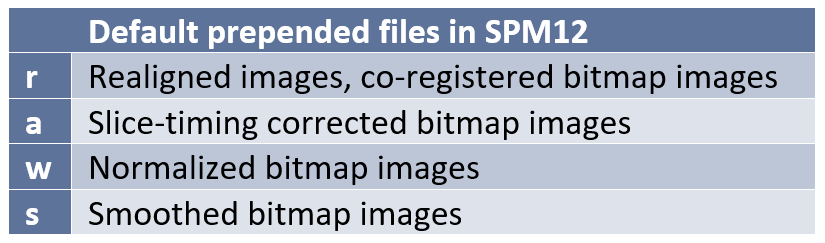
Preprocessing and File Naming Conventions in SPM12
As you are carrying out the different stages of preprocessing, SPM will automatically add (prepend) a prefix letter to the beginning of the file name to prevent overwriting previous files. Although you may designate different prefixes in the batch editor, the defaults are generally well known by SPM users and so maintaining the defaults may help others understand your dataset. The following are the default prefixes:
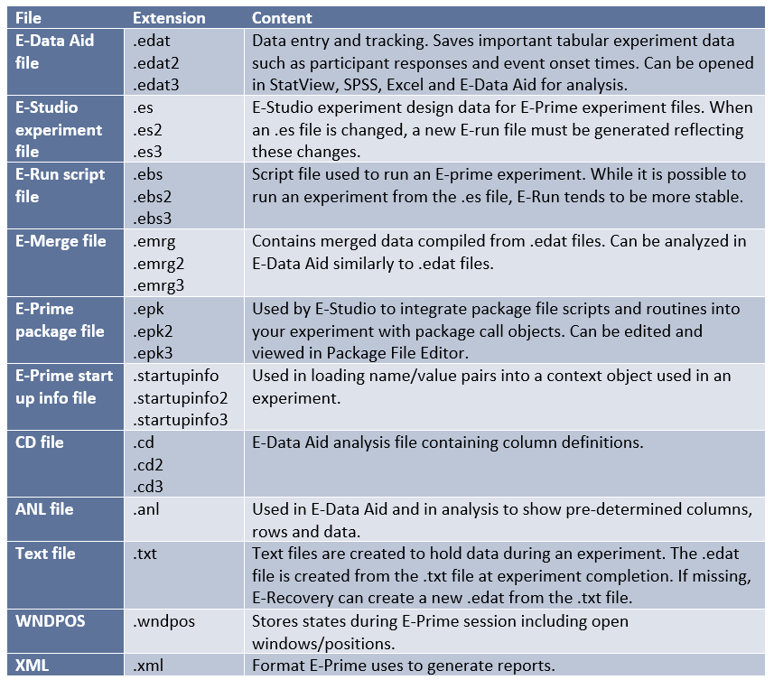
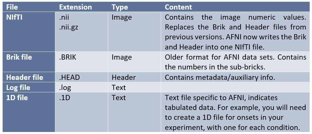
SPM12 Data Overview
The table that follows gives a very basic overview of the file types that are produced under analysis with SPM12.
AFNI
AFNI is another open source program for analysis of fMRI data. It was developed by the National Institutes of Health in the United States. One downside is that it runs only on Unix-based operating systems. Some prefer AFNI for its versatility, more fine-grained options for exploration and visualization of data and for analyzing specific types of data, such as resting state fMRI analysis. AFNI now operates with GUIs for many tasks, you may want to have some familiarity with Unix to truly utilize its features. AFNI runs with C as its primary programming language.
AFNI Data Overview
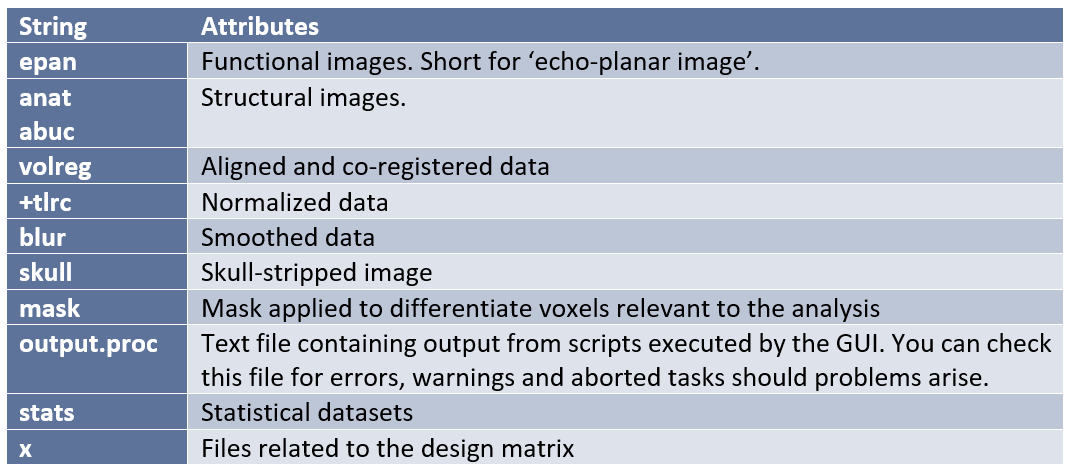
3D arrays in AFNI are called sub-bricks. There is one number per voxel in each sub-brick. Datasets are stored in directories, which are called sessions, because they contain the data from one scanning session with a participant. AFNI has its own unique set of file systems and extensions that one should be aware of when examining a dataset analyzed with the program:
AFNI has a series of strings present either in the file name or descriptors which inform the researcher of what type of image they are viewing and what preprocessing or analysis steps have been performed on them. The following are some examples:
FREESURFER
Freesurfer is an open source software for Linux and MacOS for the processing and analysis of fMRI data. Freesurfer is commonly used in preprocessing, when a researcher wants to create models from their fMRI data, and to measure the morphometric features of the brain such as regional volumes and cortical thickness. It may also be used to average intersubject structural and functional data based on cortical folds to produce alignment of different neural substrates. The program creates a 2D surface mesh from the 3D volumes to better locate sources of activation. This is helpful in cases where a particular voxel covers two different areas of the brain or two different tissue types. Boundaries are traced by the program and an inflated brain is produced, much like an brain-shaped balloon. It is also possible to further expand this inflation to the shape of a sphere for comparison across subjects. Rather than thinking about your data in terms of voxels, Freesurfer approaches the data in terms of vertices and edges (Jahn, 2019).
Parcellation is the act of labeling the different brain regions, which Freesurfer performs using two atlases, the Desikan-Killiany atlas and the Destrieux atlas. Freesurfer notoriously uses up quite a lot of processor time and memory, so you will want to run Freesurfer in an environment that supports analysis with a significant amount of processing power. Otherwise reconstruction and analysis of a large dataset can take many days. When using Freesurfer on a very large database, you may find that it is necessary to use a supercomputer. Because of these features, some researchers may find the prospect of using Freesurfer inconvenient. However, it may be worth the hassle depending on what you hope to accomplish with your fMRI data.
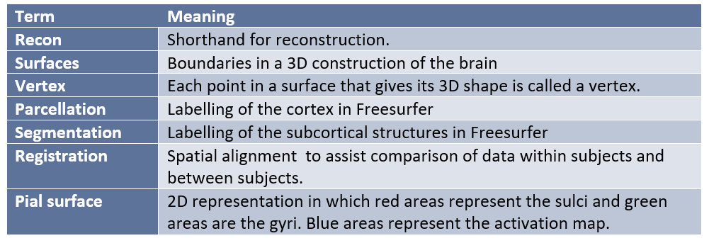
Freesurfer uses its own simple command language and jargon set that users must become acquainted with. Some examples of this jargon include:
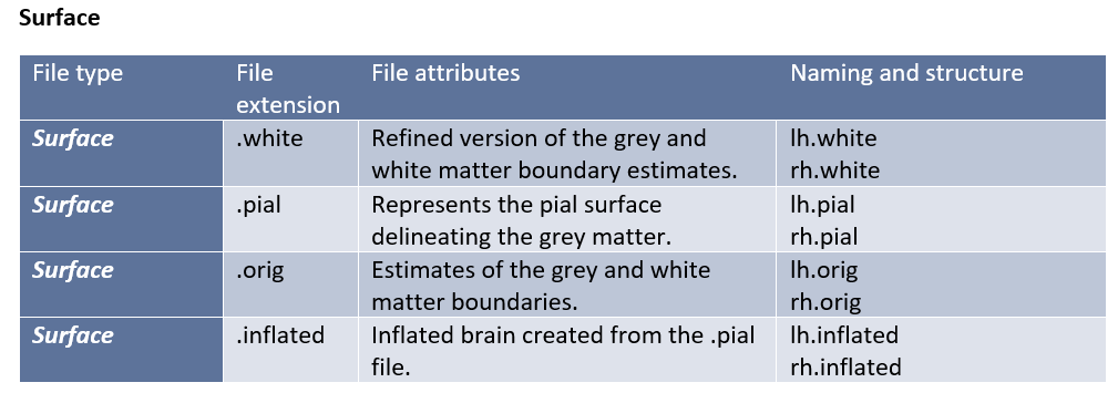
Freesurfer Data Overview
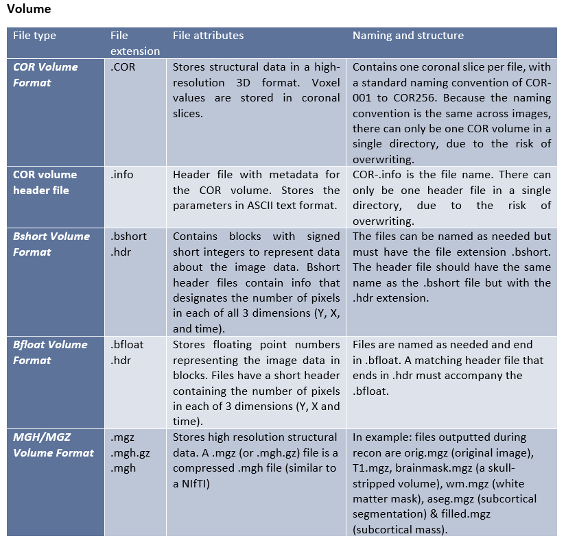
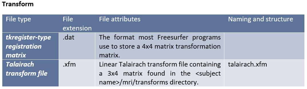
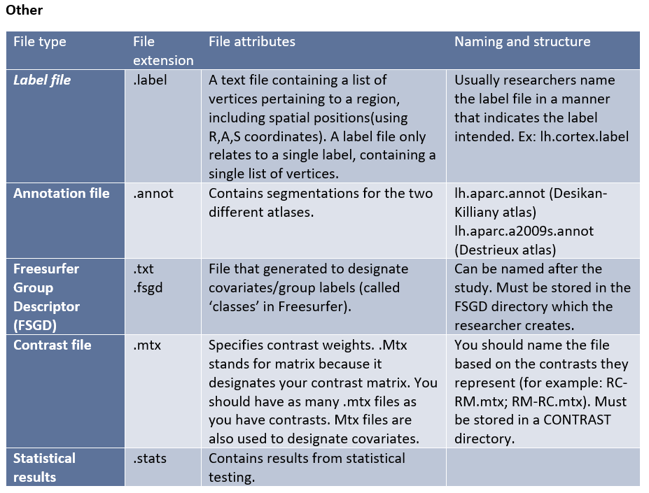
Freesurfer creates its own complex file types for different stages of the processing and analysis. These native file formats include (listed by category):
Freesurfer additionally uses its own program to view the data and analysis results, Freeview.
The program can be used to view standard formats like NIfTI, as well as the Freesurfer-specific formats generated during preprocessing and analysis.
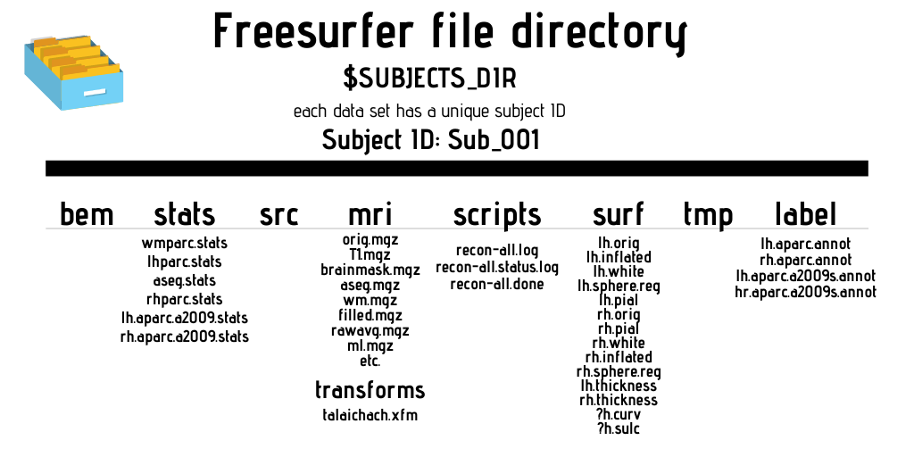
Freesurfer operates with a specific file directory schema. The $SUBJECTS_DIR contains the outputs of recon-all commands. 3D volumes are found in the ‘mri’ folder, while regions of interests and atlas annotations are found in the ‘label’ subdirectory. The ‘scripts’ directory includes log files of events that occurred while running recon-all. The ‘stats’ directory contains structural measures for the thickness and volume of each parcellation, while the ‘surf’ directory contains your surfaces, such as pial and inflated surfaces. See the directory mockup on the next page for an overview of the directory structure and the files that are commonly found within each directory.
Parts of the output file names in Freesurfer are separated by periods. Below are the most common file segments/naming conventions created by Freesurfer during analysis and what they mean in terms of the file contents:
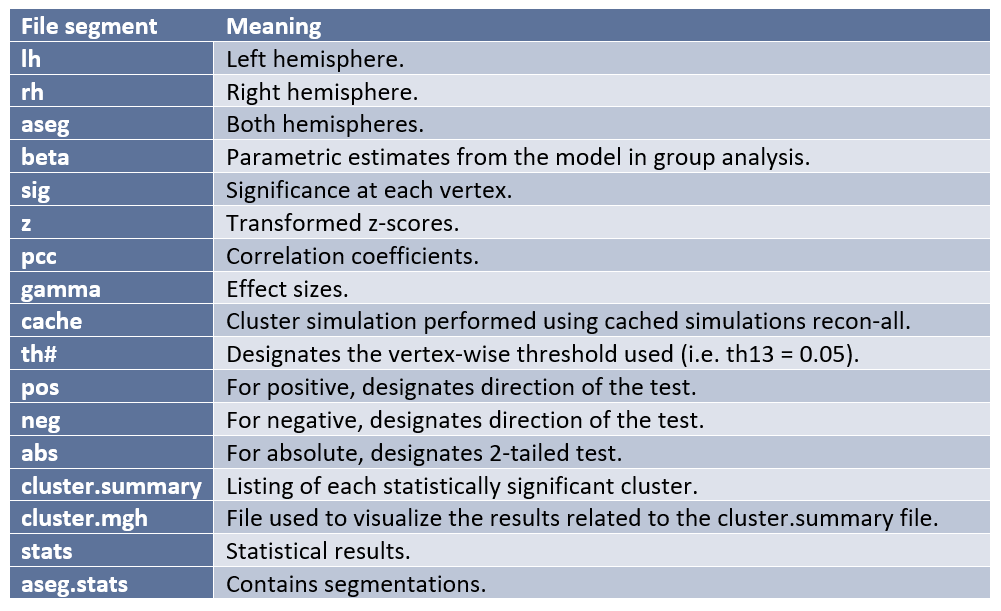
After performing second-level analysis and cluster correction (to account for multiple comparisons) the following outputs will be produced:
- Cache.th13.pos.pdf.dat
- Cache.th13.pos.sig.cluster.mgh
- Cache.th13.pos.sig.cluster.summary
- Cache.th13.pos.sig.masked.mgh
- Cache.th13.pos.sig.ocn.annot
The cluster.summary will list your statistically significant clusters and the cluster.mgh file will allow you to view your results in Freeview. (Jahn, 2019) ROI outputs, when desired, are created by Freesurfer as tab delimited text files (.txt).
FSL
FSL was created by University of Oxford. It can be used with Windows, Mac and Linux operating systems. Like AFNI, you will need to have some familiarity with Unix and a shell-like bash or tcsh to take full advantage of the program. This can be a drawback for new beginners, but it does have an easy to use GUI to assist new users. Preprocessing and analysis in FSL is performed using the application FEAT.
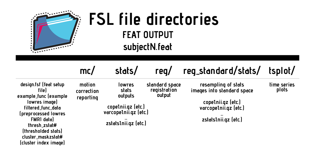
FSL Data Overview
FSL reads and produces the same file types used by SPM, namely, the NIfTI and ANALYZE standards. You will need to create your own timing/onset files in the .txt format for FSL to read. You will also need to create a separate .txt file for each condition and run. FEAT creates its own FEAT output directories for the results. For a comprehensive listing of the file structure and outputs of these directories, see https://poc.vl-e.nl/distribution/manual/fsl-3.2/feat5/output.html.
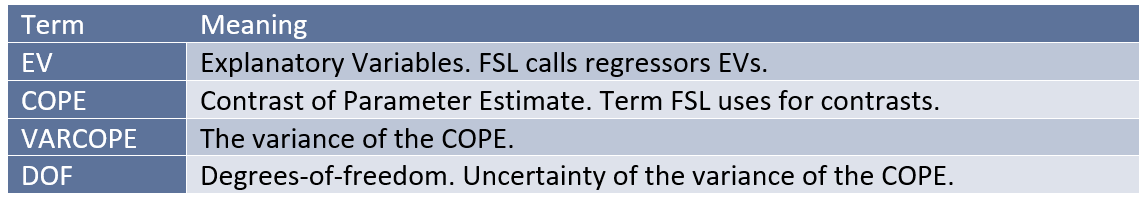
FSL also has a jargon that must be understood for the purposes of analysis and file naming conventions:
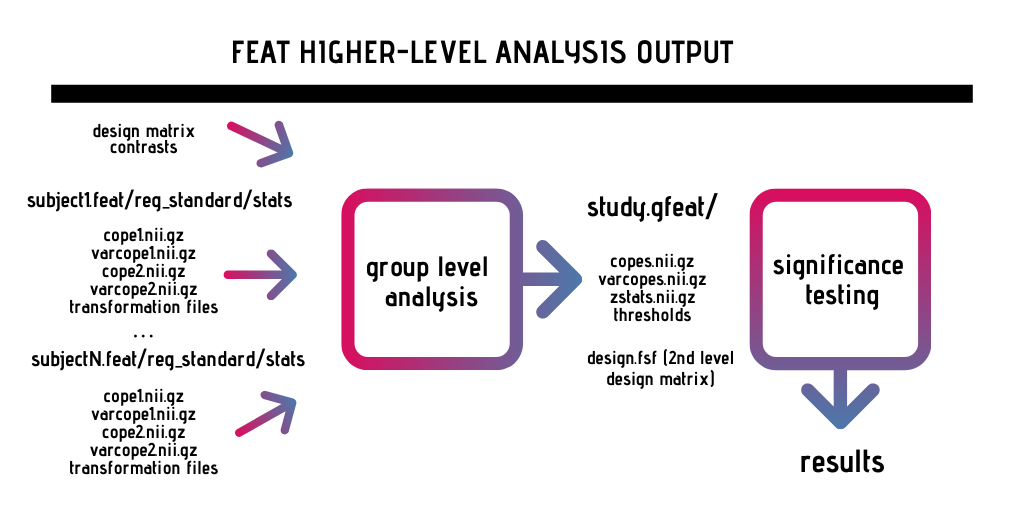
Below is a basic visualization of the different inputs/outputs related to second level analysis in FSL:
Scripting Preprocessing & First-level Analysis in SPM and FSL
Performing preprocessing and first-level analysis manually can be time-consuming and prone to error, so we recommend automatizing these tasks by writing scripts.
Scripting involves looping over and applying the same steps to all of your subjects. This requires that files are consistently labeled across subjects: functional scans, structural scans and timing files must have consistent labeling and folder structure. This is yet another reason why we recommend adopting the BIDS-format.
In general, scripting is based upon creating a template using one example subject. You then change the subject-specific references in this template to apply it to each individual subject.
Scripting for SPM
SPM is a MATLAB-based toolbox, so you will script your analysis as MATLABscripts. Scripting involves taking advantage of the "batch"-system in SPM (see the batch-button in the SPM menu), where you can specify preprocessing or statistical analysis steps.
There are two main ways of scripting in SPM:
1. Creating batches for dif erent stages of the process ("realignment", "coregistration", etc.) and saving them as .mat files (created with save batch). After, you can then loop over all your subjects, and load this .mat file for each subject. When you load it, it will show up as a variable called "matlabbatch" in MATLAB. Inside each loop (each subject), you must edit the contents of this variable, specifically all references to filenames so that they refer to the current subject, while keeping everything else the same.
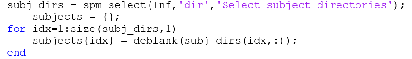
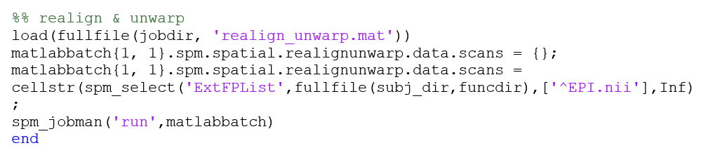
You can use spm_select to select subject directories. You can also use spm_select to make SPM find the appropriate files using a filename-filter (^EPI.nii in the example below). Spm_jobman is used to run the job (see the last line in the code below).
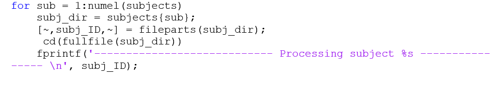
We present the following examples to demonstrate how a script might look in SPM. Here, several variables are defined earlier in the script (such as func_dir), adapted to the specific folder structure of this dataset.
Selecting subjects using spm_select and saving them as a cell array with deblanked filenames:
Looping over subjects, loading and applying .mat file – in this case performing realign&unwarp:
This approach is flexible, as you can easily edit your .mat files or save slightly different versions in the SPM batch system in the GUI.
Scripting like this involves a bit of trial and error and seeking help from experienced users, as some SPM functions require the filenames as strings, some as cells, and you have to make sure that SPM selects all volumes of the 4D EPI files and not just the first. When testing a new pipeline like this, always do one subject one step at a time and check in the “matlabbatch” variable that the right files are being selected. This will make you more intimately acquainted with what goes into the SPM functions.
If you are new to this, it is recommended that you use the “help” function in MATLAB to explore what each function does, for example typing: help spm_select
While it might be helpful to look at scripts from experienced users, beware! You should never uncritically apply a script to your own data that was intended for another dataset. Only use other researchers’ scripts to increase your understanding of SPM functions.
2. Save batch and script.
This method takes advantage of the “dependencies” option in the batch system, where you can specify multiple preprocessing steps and first level modelling in sequence. You create a batch of your pipeline specified for the files of one subject. The batch containing all the steps is saved as a .m file. Thus, you already have a matlab script and you only need to change the filenames (=subject) references. You then replace the references to the one subject with a list of your subjects and a looping variable, turning your subject-specific pipeline into a general pipeline for all subjects. This is adequately described in Andrew Jahn’s example in the link above.
Lastly, always carefully examine your data after preprocessing. Check the output of different preprocessing steps and statistical (con or T) images using the “Check Reg” function in SPM.
Scripting for FSL
FSL is based on Unix, which means that you can perform FSL functions within the terminal on a Linux or Mac, or in the FSL GUI.
The process is similar to the “save batch & script” option in SPM. In the FSL GUI, you click on FEAT fMRI analysis and select the analysis steps you want to perform. You can save this as a .fsf file, which is a subject-specific job that can be run in the terminal using the “feat” command. You can write a Unix (usually a bash) script that loops over subjects, copying this template into each subject directory (using the “cp” command) and changing the subject-specific information to the subject in the current loop (using the “sed” command), before running the job (using the “feat” command).
Andrew Jahn explains this in his tutorial, where the bash script run_1stLevel_Analysis.sh copies, edits and runs the design.fsf file.
His Unix tutorial is also recommended if you are unfamiliar with basic scripting like for-loops.