VDI – Virtual Desktop Infrastructure. Recently, VDI’s have become a popular tool for preprocessing and data analysis. VDI offers users access to a virtual computer with the software and processing power they need. This computer can be used in the same way you use your local computer but can be reached from different devices and operating systems. Which programs that are mounted and can run on the VDI machine is decided together by yourself, your local IT and program managers at the departments. A VDI may offer advantages over using one’s office desktop computer for analysis, as the VDI processing capabilities are more powerful. The lab engineer can be contacted for more information about how to connect and use UiO's VDI's.
Software
Many of the available iEEG systems come with analysis software packages with varying levels of detailed descriptions of how the different preprocessing tools are implemented. In addition, several free and commercially available software packages that run on MATLAB/Python/R platforms, offer alternative implementations of data analysis tools. At the psychology department at UiO, MATLAB is the dominant software used for iEEG data preprocessing, analysis, and visualization. MATLAB is a high-level programming environment that is relatively easy to learn and use. The mostwidely used iEEG analysis packages are MATLABbased, with the most commonly used being Fieldtrip (Oostenveld et al., 2011). MATLAB has a development environment that makes it easy to access large amounts of data. This is advantageous because one can easily inspect data during each stage of processing and analysis. One can also easily inspect and compare results from different subjects. MATLAB is also able to compute plots of your data that are customizable. These can be exported as pixel-based image files (.jpg, .bmp, .png, .tiff), vector files (.eps), or movies, which can be used to make presentations and publication-quality figures. In addition, custom-written software for preprocessing and subsequent analysis is commonly used. In-house software is usually notated by the researcher with descriptions and comments on the script..
Preprocessing and Analysis Considerations
The primary derivatives of the traditional, noninvasive scalp EEG are evoked potentials and event-related potentials. Evoked potentials (EP) are an electrical potential in following a stimulus recorded/seen in spontaneous EEG and is NOT time-locked to the event. In the case of EP, one averages the electrical activity within a specific period in which a stimulus was presented. Time-locked/event-related potentials (ERP) are measured brain responses that are a direct result of stimulus presentation and are time-locked to the event.
The iEEG records primarily local field potentials (LFP) and spike-density measures in neural activity (Lachaux et al., 2003). The cortical field potential (CFP), a recording of the activity of a local population of neurons (or the “spikes”); LFP, i.e. the direct measurement of a single or much smaller group of neurons (Fox et al., 2018); and the iERP (Lachaux et al., 2012) are the primary derivatives of iEEG. The LFP is the electrical potential that the iEEG electrodes record either subdurally or within the cortical tissue or other brain structures and is the phenomenon from which EP and ERPs are derived (Lachaux et al., 2012). Microelectrodes also have the potential to record action potentials. The spikes recorded represent the output of neurons, while the LFP represent the post-synaptic potentials, or the input of a neural population (Lauchaux et al., 2003). iERPs are calculated by event-related averaging of the LFP (Lachaux et al., 2012), while post-stimulus time histograms (PSTH) which are the iERP equivalent derived from spikes recorded by microelectrodes (Lachaux et al., 2003). iEEG can be used to study high frequency neural activity (HFA) and gamma-band responses (GBR) (Lauchaux et al., 2012). For a comprehensive description of these phenomena and how they relate to each other see Lachaux et al. 2003 and 2012.
Preprocessing Steps
The high sampling rate of iEEG data means that files are much larger than with most electrophysiological data acquisition systems. That means that for processing iEEG files, you typically will need a computer with more than the standard amount of RAM. After reading the data in MATLAB memory, a common procedure is to downsample it to reduce the sampling rate (using the ft_resampledata function in FieldTrip). [EJ1] This will make all subsequent analyses run much faster and will facilitate doing the analysis with less RAM.
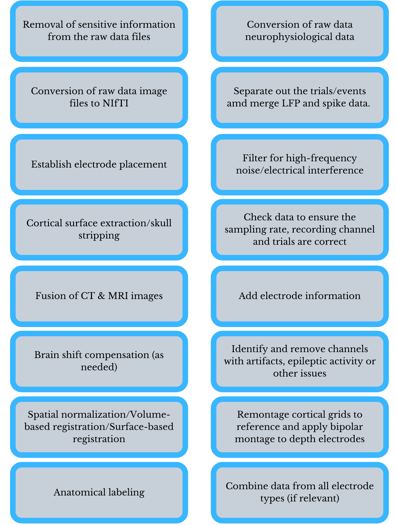
There are generally three workflows involved in processing iEEG data: handling of the MRI data and localization of electrodes/anatomical features, preprocessing of the iEEG data, and analysis itself. Unfortunately, no one program exists that is able to perform all of these steps, and thus the development of multiple workflows is often necessary (Stolk et al., 2018). The following section will provide a very basic description of the steps involved which lead up to analysis. The focus will be placed on the MATLAB-based, open-source Fieldtrip toolbox, which is not only the most widely documented program for iEEG preprocessing. For a more comprehensive description of an iEEG preprocessing and analysis protocol using Fieldtrip, see Stolk et al. (2018) and http://www.fieldtriptoolbox.org/tutorial/human_ecog/ which inform this section of the guide. Both sources also include links to a dataset that can be used as a tutorial to attempt analysis prior to working with data from your own study, as well as step by step directions and useful snippets of code.
The anatomical workflow
The anatomical data must be preprocessed, including conversion of DICOM files to the NIfTI format, defacing or skull stripping and compensating for the brain shift phenomena, spatial normalization and anatomical labeling. The anatomical data must also be coregistered, which can be performed using the most popular neuroimaging software, for example, SPM. Stolk et al. recommend the use of Freesurfer for co-registration and warping to a template, however, because the nature of how it performs these tasks, and the smoothing it performs, which can help accommodate for brain-shift and facilitate comparison across subjects (2018). For a basic guide to some of these tasks, including a brief description of the differences between SPM and Freesurfer, please see our guide Working With fMRI Data.
Electrode location must be established in concert with the anatomical scans and surgical photography, often manually, using a program like BioImage Suite or Fieldtrip with a graphical interface (Stolk et al., 2018; Fieldtrip, 2020). The electrodes must also be sorted and labeled, which can be done manually or with the use of software (Stolk et al., 2018). For the electrode placement step, you first will need to access the header information from the raw data recording file in order to create the electrode labels, which will be inputs in the electrode placement step. You will assign the locations to the different labels drawn from the header. To read the header you will use the command hdr = ft_read_header(). The anatomical data may also be warped to an atlas, a universal template brain, for comparison across subjects where possible (Stolk et al., 2018). Alternately, you may opt to use two new semi-automated MATLAB localization and visualization toolboxes for iEEG: iElvis (Groppe et al., 2017) or iElectrodes (Blenkmann et al., 2017), which was developed at UiO.
Next, work must be done to the iEEG data itself to improve the signal to noise ratio.
The signal to noise workflow
Because of the sheer size of the Neuralynx .nrd data files, when working with this system, steps must be taken to split the files into the .sdma format, which, as stated previously, splits the .nrd file into separate channels. This can be performed in Fieldtrip. All of the channel files for one session are deposited in one directory by Fieldtrip, which is able to read all files in the same session folder simultaneously.
LFPs are usually studied at a sampling rate of 512 Hz or higher. With the use of microelectrodes, the sampling rate can be as high as 30 kHz (Lachaux et al., 2003). After splitting the .nrd file, the data must be downsampled, for example, from 1,000-10,000 to 250-1,000 samples per second. Downsampling may change the temporal resolution. Downsampling solves the problem of huge data sizes that could otherwise make analysis slow and difficult. After downsampling of the data is performed, Fieldtrip allows for the data to be written into multiple non-proprietary formats, if so desired.
The data must then be segmented into epochs that correspond to the onsets of events of interest in the experiment. This is done using the event codes from the data file (Acheson, 2019). Epochs can also include an entire trial, made up of multiple events, if the data analysis strategy calls for it. It is important to understand that different file and acquisition systems can have very different time stamp definitions (Fieldtrip, 2020). These epochs will be eventually put on the same scale by averaging the signal from a short time prior to the onset, or the ‘baseline period’ and subtracting the average from every time-point in the epoch (Acheson, 2019).
The next step in preparing iEEG data for analysis is to apply a low pass and high pass filter to achieve a more smooth, defined signal. You can use the command help ft_preprocessing for assistance in applying filters to the data.[EJ1]
In the past it has been argued that iEEG is also not prone to artifacts from movement in the same way as regular EEG, however, several research teams have discovered that although the artifacts are not as severe with iEEG, they are still often present in the data (Nejedly et al., 2018). Movement artifacts may result from the fact that the patient is hooked up to wires outside the body (Parvizi & Kastner, 2018). iEEG is also not entirely immune to artifacts from muscle and eye movement (Jerbi et al., 2009; Kovach et al., 2011) or power-line interference (Nejedly et al., 2020). Movement of the electrode within the brain itself is also a consideration (Nejedly et al., 2018).
Since you are also working with a patient group which will most likely experience seizure activity during experimentation, it is also important for a clinician to annotate where seizures have occurred so that those signals can be omitted. For a description of the kinds of artifacts one might encounter with iEEG, as well as a visualization of these artifacts, see Nejedly et al., 2020. For suggestions for dealing with these eye movement artifacts see Kovach et al., 2011. Methods of locating noise and pathological activity include manual visual evaluation, independent component analysis, and more recently, convolutional neural networks (Nejedly et al., 2018).
Re-montaging (re-referencing to a different montage scheme can help remove noise occurring across channels. You may re-montage the cortical grids to a common average reference, for example. A bipolar montage may also be applied to depth electrodes. Before this is done, it is important to ensure that bad channels have been removed (Stolk et al., 2018).
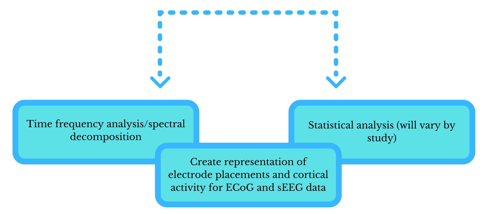
Next you want to merge the data into one data structure to make subsequent processing and analysis easier. After this, one may opt to apply a time-frequency analysis and perform interactive plotting of the data as it relates to the electrodes to allow for further analysis exploration.
For more precise tutorials on preprocessing and analysis of iEEG data using the MATLAB Fieldtrip Toolbox, see Stolk et al., 2018, as well as the following links:
Analysis of human ECoG and sEEG recordings: http://www.fieldtriptoolbox.org/tutorial/human_ecog/
Analysis of high-gamma band signals in human ECoG: http://www.fieldtriptoolbox.org/example/ecog_ny/
Preprocessing and analysis of spike and local field potential data: http://www.fieldtriptoolbox.org/tutorial/spikefield/
The exact details of analysis will vary by study, and will be based upon the research question at hand, but typically the next steps in analysis entail averaging signals in the events of interest within subjects, followed by averaging these averages across subjects, if possible, given the constraints of iEEG.
The two workflows of preprocessing (steps and order will vary)
Behavioral Data
Additional behavioral data can be acquired from the stimulus presentation software. This data can be used in conjunction with the iEEG data during analysis. Their use tends to vary according to the study’s needs. For example, you may require information about a participant's responses or response times in order to understand the patterns of activation in your iEEG data. Presentation, Psychtoolbox for MATLAB and E-Prime tend to be the most popular programs for experiments in labs, however open source programs like PsychoPy are coming more and more into use. Paradigm, PEBL, and Inquisit are additional programs for creating neuroscience experiments that you may encounter. For more information on the behavioral data you may encounter, please see our guide Working with fMRI Data.